Note
Go to the end to download the full example code.
The Benefits of Kernel PCovR for the WHO Dataset#
import numpy as np
from matplotlib import pyplot as plt
from scipy.stats import pearsonr
from sklearn.decomposition import PCA, KernelPCA
from sklearn.kernel_ridge import KernelRidge
from sklearn.linear_model import Ridge, RidgeCV
from sklearn.metrics import r2_score
from sklearn.model_selection import GridSearchCV, train_test_split

from skmatter.datasets import load_who_dataset
from skmatter.decomposition import KernelPCovR, PCovR
from skmatter.preprocessing import StandardFlexibleScaler
Load the Dataset#
df = load_who_dataset()["data"]
print(df)
           Country  Year  ...  SN.ITK.DEFC.ZS  NY.GDP.PCAP.CD
0      Afghanistan  2005  ...            36.1      255.055120
1      Afghanistan  2006  ...            33.3      274.000486
2      Afghanistan  2007  ...            29.8      375.078128
3      Afghanistan  2008  ...            26.5      387.849174
4      Afghanistan  2009  ...            23.3      443.845151
...            ...   ...  ...             ...             ...
2015  South Africa  2015  ...             5.2     6204.929901
2016  South Africa  2016  ...             5.4     5735.066787
2017  South Africa  2017  ...             5.5     6734.475153
2018  South Africa  2018  ...             5.7     7048.522211
2019  South Africa  2019  ...             6.3     6688.787271

[2020 rows x 12 columns]
Below, we take the logarithm of the population and GDP to avoid extreme distributions
log_scaled = ["SP.POP.TOTL", "NY.GDP.PCAP.CD"]
for ls in log_scaled:
    print(X_raw[:, columns.index(ls)].min(), X_raw[:, columns.index(ls)].max())
    if ls in columns:
        X_raw[:, columns.index(ls)] = np.log10(X_raw[:, columns.index(ls)])
y_raw = np.array(df["SP.DYN.LE00.IN"])
y_raw = y_raw.reshape(-1, 1)
X_raw.shape
149841.0 7742681934.0
110.460874721483 123678.70214327476

(2020, 9)
Scale and Center the Features and Targets#
x_scaler = StandardFlexibleScaler(column_wise=True)
X = x_scaler.fit_transform(X_raw)

y_scaler = StandardFlexibleScaler(column_wise=True)
y = y_scaler.fit_transform(y_raw)

n_components = 2

X_train, X_test, y_train, y_test = train_test_split(
    X, y, test_size=0.3, shuffle=True, random_state=0
)
Train the Different Linear DR Techniques#
Below, we obtain the regression errors using a variety of linear DR techniques.
Linear Regression#
0.8548848257886271
PCovR#
pcovr = PCovR(
    n_components=n_components,
    regressor=Ridge(alpha=1e-4, fit_intercept=False),
    mixing=0.5,
    random_state=0,
).fit(X_train, y_train)
T_train_pcovr = pcovr.transform(X_train)
T_test_pcovr = pcovr.transform(X_test)
T_pcovr = pcovr.transform(X)

r_pcovr = Ridge(alpha=1e-4, fit_intercept=False, random_state=0).fit(
    T_train_pcovr, y_train
)
yp_pcovr = r_pcovr.predict(T_test_pcovr).reshape(-1, 1)

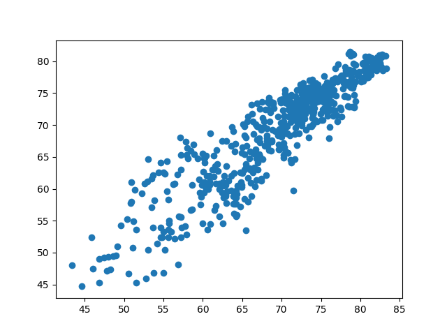
plt.scatter(y_scaler.inverse_transform(y_test), y_scaler.inverse_transform(yp_pcovr))
r_pcovr.score(T_test_pcovr, y_test)
/home/docs/checkouts/readthedocs.org/user_builds/scikit-matter/envs/284/lib/python3.13/site-packages/skmatter/decomposition/_pcov.py:62: UserWarning: This class does not automatically center data, and your data mean is greater than the supplied tolerance.
  warnings.warn(

0.8267220275787429
PCA#
pca = PCA(
    n_components=n_components,
    random_state=0,
).fit(X_train, y_train)
T_train_pca = pca.transform(X_train)
T_test_pca = pca.transform(X_test)
T_pca = pca.transform(X)

r_pca = Ridge(alpha=1e-4, fit_intercept=False, random_state=0).fit(T_train_pca, y_train)
yp_pca = r_pca.predict(T_test_pca).reshape(-1, 1)

plt.scatter(y_scaler.inverse_transform(y_test), y_scaler.inverse_transform(yp_pca))
r_pca.score(T_test_pca, y_test)

0.8041174131375703
SP.POP.TOTL -0.22694404485361058 -0.3777743593940685
SH.TBS.INCD -0.6249287177098702 0.6316215151702457
SH.IMM.MEAS 0.8425862283813431 0.1360690482747262
SE.XPD.TOTL.GD.ZS 0.4145734240484015 0.6100854823971252
SH.DYN.AIDS.ZS -0.3260933054303096 0.8499296260662147
SH.IMM.IDPT 0.8422637385674645 0.1633976966291517
SH.XPD.CHEX.GD.ZS 0.4590012089554525 0.3068630393788186
SN.ITK.DEFC.ZS -0.8212324937958553 0.05510883584395139
NY.GDP.PCAP.CD 0.8042167907410394 0.06566227478694865
Train the Different Kernel DR Techniques#
Below, we obtain the regression errors using a variety of kernel DR techniques.
Select Kernel Hyperparameters#
In the original publication, we used a cross-validated grid search to determine the
best hyperparameters for the kernel ridge regression. We do not rerun this expensive
search in this example but use the obtained parameters for gamma and alpha.
You may rerun the calculation locally by setting recalc=True.
recalc = False

if recalc:
    param_grid = {"gamma": np.logspace(-8, 3, 20), "alpha": np.logspace(-8, 3, 20)}

    clf = KernelRidge(kernel="rbf")
    gs = GridSearchCV(estimator=clf, param_grid=param_grid)
    gs.fit(X_train, y_train)

    gamma = gs.best_estimator_.gamma
    alpha = gs.best_estimator_.alpha
else:
    gamma = 0.08858667904100832
    alpha = 0.0016237767391887243

kernel_params = {"kernel": "rbf", "gamma": gamma}
Kernel Regression#
KernelRidge(**kernel_params, alpha=alpha).fit(X_train, y_train).score(X_test, y_test)
0.9726524136785997
KPCovR#
kpcovr = KernelPCovR(
    n_components=n_components,
    regressor=KernelRidge(alpha=alpha, **kernel_params),
    mixing=0.5,
    **kernel_params,
).fit(X_train, y_train)

T_train_kpcovr = kpcovr.transform(X_train)
T_test_kpcovr = kpcovr.transform(X_test)
T_kpcovr = kpcovr.transform(X)

r_kpcovr = KernelRidge(**kernel_params).fit(T_train_kpcovr, y_train)
yp_kpcovr = r_kpcovr.predict(T_test_kpcovr)

plt.scatter(y_scaler.inverse_transform(y_test), y_scaler.inverse_transform(yp_kpcovr))
r_kpcovr.score(T_test_kpcovr, y_test)

0.9701003539460146
KPCA#
kpca = KernelPCA(n_components=n_components, **kernel_params, random_state=0).fit(
    X_train, y_train
)

T_train_kpca = kpca.transform(X_train)
T_test_kpca = kpca.transform(X_test)
T_kpca = kpca.transform(X)

r_kpca = KernelRidge(**kernel_params).fit(T_train_kpca, y_train)
yp_kpca = r_kpca.predict(T_test_kpca)

plt.scatter(y_scaler.inverse_transform(y_test), y_scaler.inverse_transform(yp_kpca))
r_kpca.score(T_test_kpca, y_test)

0.6661226058827718
Correlation of the different variables with the KPCovR axes#
SP.POP.TOTL 0.07320109486753514 0.03969226130180457
SH.TBS.INCD 0.6836177728806975 -0.053847467714366354
SH.IMM.MEAS -0.6604939713030814 0.04751969851825911
SE.XPD.TOTL.GD.ZS -0.23009788930020497 -0.3622748866000346
SH.DYN.AIDS.ZS 0.5157981075022396 -0.11701327000295882
SH.IMM.IDPT -0.6449500965012945 0.052622267818724124
SH.XPD.CHEX.GD.ZS -0.3801993556012609 -0.5736426627623825
SN.ITK.DEFC.ZS 0.7301250686596557 0.047934542867408364
NY.GDP.PCAP.CD -0.8228660097330227 -0.49386365697106455
Plot Our Results#
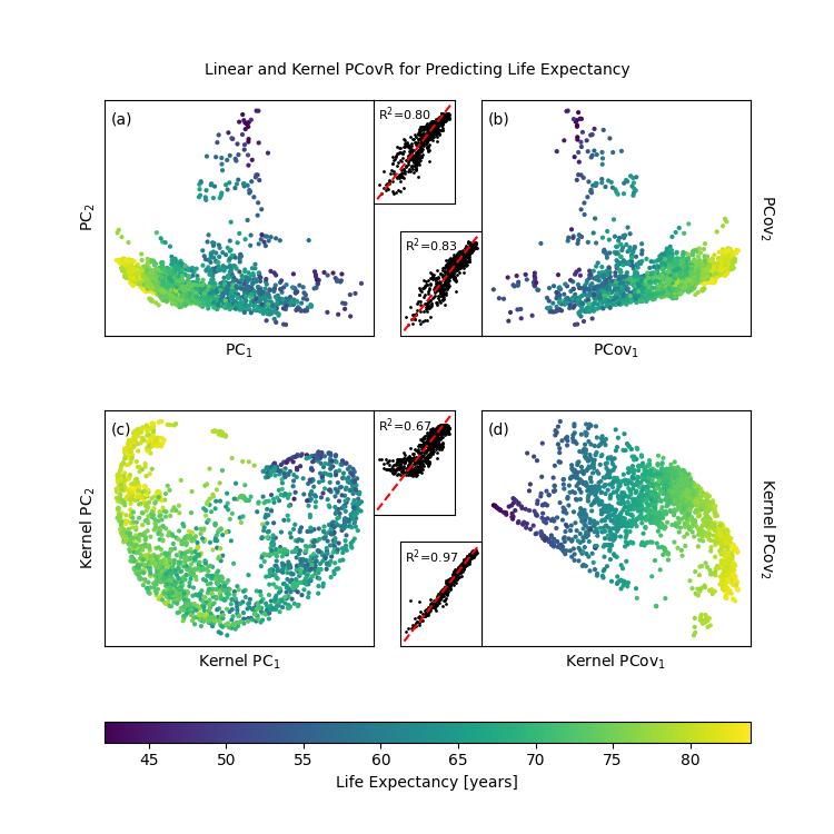
fig, axes = plt.subplot_mosaic(
    """
                                AFF.B
                                A.GGB
                                .....
                                CHH.D
                                C.IID
                                .....
                                EEEEE
                                """,
    figsize=(7.5, 7.5),
    gridspec_kw=dict(
        height_ratios=(0.5, 0.5, 0.1, 0.5, 0.5, 0.1, 0.1),
        width_ratios=(1, 0.1, 0.2, 0.1, 1),
    ),
)
axPCA, axPCovR, axKPCA, axKPCovR = axes["A"], axes["B"], axes["C"], axes["D"]
axPCAy, axPCovRy, axKPCAy, axKPCovRy = axes["F"], axes["G"], axes["H"], axes["I"]


def add_subplot(ax, axy, T, yp, let=""):
    """Adding a subplot to a given axis."""
    p = ax.scatter(-T[:, 0], T[:, 1], c=y_raw, s=4)
    ax.set_xticks([])
    ax.set_yticks([])
    ax.annotate(
        xy=(0.025, 0.95), xycoords="axes fraction", text=f"({let})", va="top", ha="left"
    )
    axy.scatter(
        y_scaler.inverse_transform(y_test),
        y_scaler.inverse_transform(yp),
        c="k",
        s=1,
    )
    axy.plot([y_raw.min(), y_raw.max()], [y_raw.min(), y_raw.max()], "r--")
    axy.annotate(
        xy=(0.05, 0.95),
        xycoords="axes fraction",
        text=r"R$^2$=%0.2f" % round(r2_score(y_test, yp), 3),
        va="top",
        ha="left",
        fontsize=8,
    )
    axy.set_xticks([])
    axy.set_yticks([])
    return p


p = add_subplot(axPCA, axPCAy, T_pca, yp_pca, "a")
axPCA.set_xlabel("PC$_1$")
axPCA.set_ylabel("PC$_2$")

add_subplot(axPCovR, axPCovRy, T_pcovr @ np.diag([-1, 1]), yp_pcovr, "b")
axPCovR.yaxis.set_label_position("right")
axPCovR.set_xlabel("PCov$_1$")
axPCovR.set_ylabel("PCov$_2$", rotation=-90, va="bottom")

add_subplot(axKPCA, axKPCAy, T_kpca @ np.diag([-1, 1]), yp_kpca, "c")
axKPCA.set_xlabel("Kernel PC$_1$", fontsize=10)
axKPCA.set_ylabel("Kernel PC$_2$", fontsize=10)

add_subplot(axKPCovR, axKPCovRy, T_kpcovr, yp_kpcovr, "d")
axKPCovR.yaxis.set_label_position("right")
axKPCovR.set_xlabel("Kernel PCov$_1$", fontsize=10)
axKPCovR.set_ylabel("Kernel PCov$_2$", rotation=-90, va="bottom", fontsize=10)

plt.colorbar(
    p, cax=axes["E"], label="Life Expectancy [years]", orientation="horizontal"
)
fig.subplots_adjust(wspace=0, hspace=0.4)
fig.suptitle(
    "Linear and Kernel PCovR for Predicting Life Expectancy", y=0.925, fontsize=10
)
plt.show()